UCI 머신러닝 리포지토리에서 제공하는 사용자 행동 인식(Human Activity Recognition) 데이터 세트를 활용하여 결정트리를 실습해보았다.
해당 데이터 셋은 30명의 스마트 폰 센서를 장착한 뒤, 사람의 동작과 관련된 여러가지 피처를 수집한 데이터로써, 그것이 어떤 동작인지 예측해야 한다. 주어진 데이터 셋에는 features.txt(피처의 이름 기술)와 train용도의 피처 데이터 세트와 레이블 데이터 세트, 테스트용 피처 데이터 세트와 레이블 데이터 세트가 들어있다.
가장 먼저, features.txt를 불러와 피처의 갯수와 값들을 알아보았다.
import pandas as pd
import matplotlib.pyplot as plt
%matplotlib inline

# feature.txt 파일에는 피처 이름 index와 피처명이 공백으로 분리되어져 있음. 이를 DataFrame으로 로드
feature_name_df = pd.read_csv("/content/drive/MyDrive/스터디 공부/dataset/human_activity/features.txt", sep = '\s+',
                              header = None, names = ['column_index', 'column_name'])

# 피처명 index를 제거하고, 피처명만 리스트 객체로 생성한 뒤 샘플로 10개만 추출
feature_name = feature_name_df.iloc[:,1].values.tolist()
print('전체 피처명에서 10개만 추출:', feature_name[:10])


# output
전체 피처명에서 10개만 추출: ['tBodyAcc-mean()-X', 'tBodyAcc-mean()-Y', 'tBodyAcc-mean()-Z', 'tBodyAcc-std()-X', 'tBodyAcc-std()-Y', 'tBodyAcc-std()-Z', 'tBodyAcc-mad()-X', 'tBodyAcc-mad()-Y', 'tBodyAcc-mad()-Z', 'tBodyAcc-max()-X']
피처명을 보았을 때 움직임과 관련된 속성의 평균, 표준편차가 x,y,z축 값으로 되어 있음을 유추할 수 있다.
이를 데이터 프레임으로 변환하기 전에, 중복된 피처명에 대해서 구분지어주어야 한다.
# 중복된 피처명이 있는지 알아보기
feature_dup_df = feature_name_df.groupby('column_name').count()
print(feature_dup_df[feature_dup_df['column_index']>1].count())
feature_dup_df[feature_dup_df['column_index']>1].head()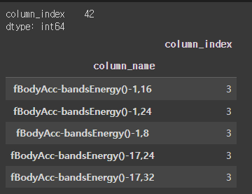
중복된 피처명이 총 42개가 존재하고, 각각의 갯수들을 확인할 수 있다.
이러한 중복된 피처명에 _1,_2를 추가로 부여해 새로은 데이터프레임을 가지는 get_new_feature_name_df()를 생성하였다.
# 중복된 피처명에 _1, _2를 추가하여 새로운 피처명을 가지는 dataframe으로 반환하는 함수 생성

def get_new_feature_name_df(old_feature_name_df):
  feature_dup_df = pd.DataFrame(data = old_feature_name_df.groupby('column_name').cumcount(),
                                columns = ['dup_cnt'])
  feature_dup_df = feature_dup_df.reset_index()
  new_feature_name_df = pd.merge(old_feature_name_df.reset_index(), feature_dup_df, how = 'outer')
  new_feature_name_df['column_name'] = new_feature_name_df[['column_name',
                                                             'dup_cnt']].apply(lambda x : x[0]+'_'+str(x[1])
                                                             if x[1] > 0 else x[0] , axis = 1)
  new_feature_name_df = new_feature_name_df.drop(['index'], axis = 1)
  return new_feature_name_df
get_new_feature_name_df를 생성해준 뒤, features.txt 속성에 적용시켜주고, 데이터 셋에 있는 train, test 파일의 피처 데이터 파일과 레이블 데이터 파일을 불러와준다.
레이블 데이터 파일의 레이블 속성은 'action'으로 지정해주고, get_new_feature_df 함수를 적용시켜 데이터프레임을 만드는 일이 종종 발생하기 때문에 이를 적용시켜주는 get_human_dataset() 함수를 새롭게 생성해준다.
import pandas as pd

def get_human_dataset( ):

  # 각 데이터 파일은 공백으로 분리되어 있으므로 read_csv에서 공백 문자를 sep으로 할당
  feature_name_df = pd.read_csv("/content/drive/MyDrive/스터디 공부/dataset/human_activity/features.txt", sep = '\s+',
                                header = None, names = ['column_index','column_name'])
  # 중복된 피처명을 수정하는 get_new_feature_name_df()를 이용, 신규 피처명 DataFrame 생성
  new_feature_name_df = get_new_feature_name_df(feature_name_df)

  # DataFrame에 피처명을 칼럼으로 부여하기 위해 리스트 객체로 다시 변환
  feature_name = new_feature_name_df.iloc[:,1].values.tolist()

  # 학습 피처 데이터세트와 테스트 피처 데이터를 DataFrame으로 로딩. 칼럼명은 feature_name 적용
  X_train = pd.read_csv("/content/drive/MyDrive/스터디 공부/dataset/human_activity/train/X_train.txt", sep = '\s+', names = feature_name)
  X_test = pd.read_csv("/content/drive/MyDrive/스터디 공부/dataset/human_activity/test/X_test.txt", sep = '\s+', names = feature_name)

  # 학습 레이블과 테스트 레이블 데이터를 DataFrame으로 로딩하고 칼럼명은 action으로 부여
  y_train = pd.read_csv("/content/drive/MyDrive/스터디 공부/dataset/human_activity/train/y_train.txt", sep = '\s+', header = None, names = ['action'])
  y_test = pd.read_csv("/content/drive/MyDrive/스터디 공부/dataset/human_activity/test/y_test.txt",sep = '\s+', header = None, names = ['action'])

  # 로드된 학습/테스트용 DataFrame을 모두 반환
  return X_train, X_test, y_train, y_test

X_train, X_test, y_train, y_test = get_human_dataset()
결론적으로 모델을 생성하기 전에 데이터 셋을 분리해주어야 하는데, 분리하는 것까지 포함한 get_human_dataset()을 데이터 셋 분리할 때 적용시켜주었다.
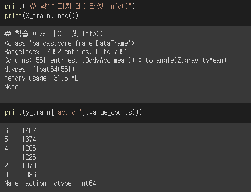
데이터 셋을 확인해보면, 학습 데이터 셋에는 7352개의 값과 561개의 피처를 가지고 있으며 모두 float 형태이기 때문에 인코딩을 진행시켜 주지 않아도 된다.
테스트 데이터 셋에는 1 ~ 6까지의 레이블이 존재한다.
DecisionTreeClassifier를 불러온 뒤 기본 파라미터를 이용하여 데이터를 학습, 예측을 해주었다.
결론적으로 정확도와 기본 하이퍼 파라미터에 해당하는 값에 어떤 값을 사용했는지 출력해보았다.
# 의사결정나무로 분류하기
from sklearn.tree import DecisionTreeClassifier
from sklearn.metrics import accuracy_score

# 예제 반복 시마다 동일한 예측 결과 도출을 위해 random_state 설정
dt_clf = DecisionTreeClassifier(random_state = 156)
dt_clf.fit(X_train, y_train)
pred = dt_clf.predict(X_test)
accuracy = accuracy_score(y_test, pred)
print("결정트리 예측 정확도: {0:.4f}".format(accuracy))

# DecisionTreeClassifier의 하이퍼 파라미터 추출
print("DecisionTreeClassifier 기본 하이퍼 파라미터:\n", dt_clf.get_params())


# output
결정트리 예측 정확도: 0.8548
DecisionTreeClassifier 기본 하이퍼 파라미터:
 {'ccp_alpha': 0.0, 'class_weight': None, 'criterion': 'gini', 'max_depth': None, 'max_features': None, 'max_leaf_nodes': None, 'min_impurity_decrease': 0.0, 'min_samples_leaf': 1, 'min_samples_split': 2, 'min_weight_fraction_leaf': 0.0, 'random_state': 156, 'splitter': 'best'}
결정트리의 하이퍼 파라미터 중 max_depth의 최적값을 찾기 위해 값을 변화 시키면서 예측성능을 확인해보았다. min_samples_split은 16으로 고정하였다.
# GridSearchCV 실행
from sklearn.model_selection import GridSearchCV

params = {
    'max_depth' : [6,8,10,12,16,20,24],
    'min_samples_split' : [16]
}

grid_cv = GridSearchCV(dt_clf, param_grid = params, scoring = 'accuracy', cv = 5, verbose = 1)
grid_cv.fit(X_train, y_train)
print('GridSearchCV 최고 평균 정확도 수치: {0:.4f}'.format(grid_cv.best_score_))
print('GridSearchCV 최적 하이퍼 파라미터:', grid_cv.best_params_)


## output
Fitting 5 folds for each of 7 candidates, totalling 35 fits
GridSearchCV 최고 평균 정확도 수치: 0.8549
GridSearchCV 최적 하이퍼 파라미터: {'max_depth': 8, 'min_samples_split': 16}
# GridSearchCV 객체의 cv_results_ 속성을 DataFrame으로 생성
cv_results_df = pd.DataFrame(grid_cv.cv_results_)
# max_depth 파라미터 값과 그때의 테스트 세트, 학습 데이터 세트의 정확도 수치 추출
cv_results_df[['param_max_depth', 'mean_test_score']]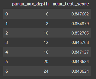
결론적으로 max_depth 가 8일때, 모델의 정확도 성능이 0.8548에서 0.8549로 상승한 것을 알 수 있다.
다음으로 별도의 테스트 데이터 셋에서 minsamples_split은 16으로 고정하고, max_depth의 변화에 따른 값을 측정해보았다.
max_depths = [6,8,10,12,16,20,24]
# max_depth 값을 변화시키면서 그때마다 학습과 테스트 세트에서의 예측 성능 측정
for depth in max_depths:
  dt_clf = DecisionTreeClassifier(max_depth = depth, min_samples_split = 16, random_state = 156)
  dt_clf.fit(X_train, y_train)
  pred = dt_clf.predict(X_test)
  accuracy = accuracy_score(y_test, pred)
  print('max_depth = {0} 정확도: {1:.4f}'.format(depth, accuracy))


  # ouput
max_depth = 6 정확도: 0.8551
max_depth = 8 정확도: 0.8717
max_depth = 10 정확도: 0.8599
max_depth = 12 정확도: 0.8571
max_depth = 16 정확도: 0.8599
max_depth = 20 정확도: 0.8565
max_depth = 24 정확도: 0.8565
테스트 데이터 셋에서도 mox_depth가 8일 때 87.17%로 가장 성능이 좋게 나왔다.
다음으로는 min_samples_split도 변화를 주면서 정확도 성능을 튜닝해보았다.
params = {
    'max_depth' : [6,8,10,12,16,20,24],
    'min_samples_split' : [16, 24]
}

grid_cv = GridSearchCV(dt_clf, param_grid = params, scoring = 'accuracy', cv = 5, verbose = 1)
grid_cv.fit(X_train, y_train)
print('GridSearchCV 최고 평균 정확도 수치: {0:.4f}'.format(grid_cv.best_score_))
print('GridSearchCV 최적 하이퍼 파라미터:', grid_cv.best_params_)


# output
GridSearchCV 최고 평균 정확도 수치: 0.8549
GridSearchCV 최적 하이퍼 파라미터: {'max_depth': 8, 'min_samples_split': 16}
best_estimator_을 이용하여 테스트 데이터 셋의 최고 정확도가 무엇인지 알아보았다.
best_df_clf = grid_cv.best_estimator_
pred1 = best_df_clf.predict(X_test)
accuracy = accuracy_score(y_test, pred1)
print('결정트리 예측 정확도:{0:.4f}'.format(accuracy))


# output
결정트리 예측 정확도:0.8717
마지막으로 결정 트리에서 각 피처의 중요도를 feature_importances_ 속성을 이용해 알아보았다.
import seaborn as sns

ftr_importances_values = best_df_clf.feature_importances_
# Top 중요도로 정렬을 쉽게 하고, 시본의 막대그래프로 쉽게 표현하기 위해 Series 변환
ftr_importances = pd.Series(ftr_importances_values, index = X_train.columns)
# 중요도값 순으로 Series를 정렬
ftr_top20 = ftr_importances.sort_values(ascending = False)[:20]
plt.figure(figsize = (8,6))
plt.title('Feature importances Top 20')
sns.barplot(x = ftr_top20, y = ftr_top20.index)
plt.show()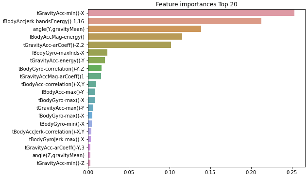
'Data Analysis > Python' 카테고리의 다른 글
| 분류_GBM(Gradient Boost Machine) (0) | 2023.02.01 |
|---|---|
| 분류_앙상블 학습 (0) | 2023.02.01 |
| 분류_결정트리(DecisonTreeClassifier) (0) | 2023.01.31 |
| 타이타닉 생존자 예측 (with 사이킷런) (0) | 2023.01.11 |
| 스케일링 및 정규화 (0) | 2023.01.11 |


